As part of my fun winter break activities I decided to write a simple package porting SAS-like formats to help practice my “test driven development” as well as continue to improve my R skills. Whilst creating it I ended up going down two different rabbit holes which I hope to cover in this post. The package can be found and installed from github at tomratford/SASformatR.

A whistle-stop tour of the package⌗

The package tries to port the idea of how SAS formats are created. There is very simple functionality for ranges of numeric values and all the standard enum -> enum formats.

library(SASformatR)

proc_format(
  PARAMCD = value(
    "SYSBP" = "Systolic Blood Pressure",
    "HR" = "Heart Rate"
  ),
  AGEGR1 = value(
    "<21" = "<21",
    "21 - 39" = "21 - 39",
    "40<=" = ">=40"
  )
)

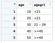
We can then use put() to format these values straight to character, or use SASformat() to create a new S3 SASformat object.

age <- seq(10,50,10)

put(age,"AGEGR1")
#> [1] "<21"     "<21"     "21 - 39" ">=40"    ">=40"

dplyr::bind_rows(age = age, agegr1 = SASformat(age,"AGEGR1"))
#> # A tibble: 5 × 2
#>     age agegr1    
#>   <dbl> <SASformt>
#> 1    10 <21       
#> 2    20 <21       
#> 3    30 21 - 39   
#> 4    40 >=40      
#> 5    50 >=40

The SASformat object has the same underlying type, so regular arithmetic can be used.

agegr1 <- SASformat(age, "AGEGR1")

class(agegr1)
#> [1] "SASformat"

typeof(agegr1)
#> [1] "double"

agegr1
#> [1] "<21"     "<21"     "21 - 39" ">=40"    ">=40"
agegr1 + 10
#> [1] "<21"     "21 - 39" ">=40"    ">=40"    ">=40"

The key purpose was to try to mimic (as much as possible) SAS formats. proc_format() does not return anything, it instead creates a format catalogue as a side effect. Another key thing to note is that this catalog is not stored in the environment it is called in.

my_new_env <- new.env()
with(my_new_env,
     {
       i_am_here <- 1
       proc_format()
     })
ls(envir = my_new_env)
#> [1] "i_am_here"

Using enviroments as mutable package data⌗

R has the ability to export data in a package. Typically this is used for exporting data frames for use in examples or vignettes. These are immutable structures, for example, if we try to assign using the :: operator we will get an error back.

dplyr::starwars <- mtcars
#> Error in dplyr::starwars <- mtcars: object 'dplyr' not found

Using the more involved assign will also not work, but will give us a more useful error message.

assign("starwars", NULL, envir = as.environment("package:dplyr"))
#> Error in assign("starwars", NULL, envir = as.environment("package:dplyr")): cannot change value of locked binding for 'starwars'

However, the exported ‘data’ can be of any type. In SASformatR I export a empty environment, this is where the format catalogues will live.

## code to prepare `ctl` dataset goes here

ctls <- new.env(parent = emptyenv())

usethis::use_data(ctls, overwrite = TRUE)

This can then be accessed from other functions within the package using SASformat::ctls. For example, within the function proc_format().

proc_format <- function(..., catalog = "formats") {
  partial <- SASformatR::ctls[[catalog]]
  if (is.null(SASformatR::ctls[[catalog]])) {
    partial <- list()
  }

  newlist <- c(list2(...), partial)

  assign(catalog,
         newlist[!duplicated(names(newlist))],
         envir = SASformatR::ctls)
}

Firstly we get the current values within the catalog, and then combine these with the new values provided to the function. The key code here is the last assign(), where I assign this new list of formats to the SASformatR::ctls environment with the name of the desired catalog - "formats" by default.

This allows formats to remain hidden from the main environment, which means it is perfectly possible to reuse names without fear of conflicts. Equally having a consistent area for formats means that we do not need to worry about load order or name conflicts within other packages, as we can explicitly specify the location.

proc_format(catalog = "EMA",
  agegr1 = value(
    "<21" = "< 21",
    "21 - 39" = "21 - 39",
    "40<=" = ">= 40"
  )
)
proc_format(catalog = "FDA",
  agegr1 = value(
    "<18" = "< 18",
    "18 - 39" = "18 - 39",
    "40 - 79" = "40 - 79",
    "80<=" = ">= 80"
  )
)

EMA <- SASformat(age, "agegr1", "EMA")
FDA <- SASformat(age, "agegr1", "FDA")
agegr1 <- dplyr::bind_cols(AGEGR1 = EMA, AGEGR2 = FDA)
agegr1
#> # A tibble: 5 × 2
#>   AGEGR1     AGEGR2    
#>   <SASformt> <SASformt>
#> 1 < 21       < 18      
#> 2 < 21       18 - 39   
#> 3 21 - 39    18 - 39   
#> 4 >= 40      40 - 79   
#> 5 >= 40      40 - 79

Aside: These are not the standard EMA and FDA age groupings but they serve the purpose of an real-world example

Custom rendering of S3 classes within a View() command⌗

Another thing which I desperately wanted to have was to be able to see the formatted values when using the View() command. This is actually very simple (but it was quite annoying to find out). Your S3 object needs a method for format() and [ (I imagine this will also work for S4 objects but I haven’t tested this). For those unaware, `[`() is the function that is called when you do something like x[1], you can actually call it like `[`(x,1). Here is the implementations within SASformatR.

`[.SASformat` <- function(x, ...) {
  structure(NextMethod(),
            class = class(x),
            format = attr(x, "format"),
            catalog = attr(x, "catalog"))
}

As we are not changing the values underneath, we can just call NextMethod() to get the base implementation for vectors. We can then reapply the attributes of our class using the structure() command.

format.SASformat <- function(x, ...) {
  check_sasformat(x) # in case of changes to the catalog
  put(unclass(x),
      attr(x,"format"),
      attr(x,"catalog"))
}

This uses the put() command that was created before.

With these two methods created we can now view our rendered values within Rstudio’s View() function, for example

my_df <- dplyr::bind_rows(age = age, agegr1 = SASformat(age,"AGEGR1"))
View(my_df)