To celebrate the completion of my MSc in statistics, and my return back to the working world, I’ve written this blog post to discuss the tools I used whilst studying. Primarily, this will be focused on my use of logseq, zotero, and emacs¹ to write my MSc dissertation. Logseq was my “second brain” throughout the year. A “second brain” is a concept popularised by Thiago Forte, and is a method for capturing and distilling relevant information from sources for the purpose of writing about them later on. I’m not sure my second brain truly represents this concept and it instead may be closer to the “Zettelkasten” method, in which you focus on smaller individual cards of research which are grouped together by metadata and tags. Zettelkasten is German for slip box, as the pre-digital act involved storing paper notes/cutouts in smaller, grouped boxes. Either of these methods can be implemented using a number of different apps, including (but not limited to)

• Logseq
• Notion
• Obsidian
• Roam Research
• Evernote
• Mem.ai
• Reflect notes
• Supernotes

and many more. I chose Logseq because it was the first one I tried, as an added plus it is FOSS software and everything I write is stored and backed up on my machine.

Zotero is a reference manager, it was chosen due to it’s interoperability with logseq.

Emacs is my text editor of choice, I have an extensive init.el generated from an literal .org file that can be found on my github.

I think I’ve gone mad⌗

In my undergraduate degree, I took notes primarly by either rewriting the notes by hand, or printing off and highlighting notes as I listened to the lectures. This helped me stay engaged (as much as possible), but generally resulted in me having a set of useless notes when it came to exam revision. Instead my aim this time round was to write notes in Logseq with each element of the content having it’s own page. As opposed to writing up an entire lecture on 2-3 pages and then not being able to refer back to it easily later. Furthermore, having taken three years out between my undergraduate and postgraduate degree my statistics knowledge was very rusty, and I knew that being able to quickly find and recap information mid-lecture would help mitigate some of this rust. My university provided sets of lecture notes in advance to refresh my knowledge, and my second brain began on June 12th, nearly four months before my first lecture. This gave me lots of time to get used to the note taking procedure, particularly refreshing my knowledge of \(\LaTeX\).

Logseq’s \(\LaTeX\) implementation, via KaTeX, is somewhat restrictive. For example, you cannot easily set commands for common symbols - such as simplifying \(\mathbb{E}\) to \E or allowing you to wrap \[ \begin{align*} H_0: \theta_{0} = 0 && \text{ vs. } &&& H_1: \theta_{0} \ne 0 \end{align*} \] to \HTest{\theta_0 = 0}{\theta_0 \ne 0}. Logseq has the ability to execute custom javascript code (being an electron app) at the rendering time which allows you to, with quite a bit of hacking, write your own custom KaTeX macros. This massively helped me speed up my note taking; particularly a macro for writing the partial derivatives was very useful when writing out larger Fisher information matrices while ensuring legibility.

Over the year I wrote ~125,000 words across 762 pages into my second brain. Each of these pages can be referenced using square brackets, e.g. writing ...we can use the [[Delta Method]] to estimate the variance... links a page to the “Delta Method” page. On the “Delta Method” page itself a “backlink” shows where it has been referenced. Logseq’s design (based of the design of Roam research) is also based on each “block” of the content being it’s own entity, such that you can reference a specific part of a specific page inline, allowing you to create networks of linked pages and avoid rewriting the same information. For example below on my page for sample size calculations, I link directly to information on my page on power. I can edit the page on power directly from this linked block, it is not read-only. 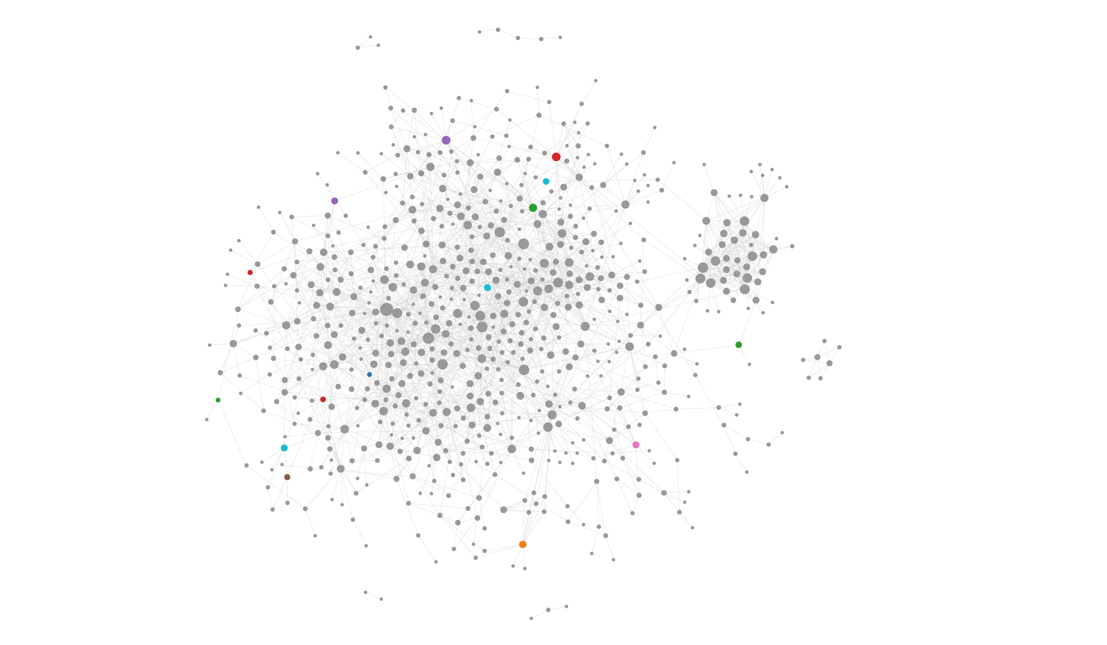My full knowledge graph can be seen at the bottom of this post.

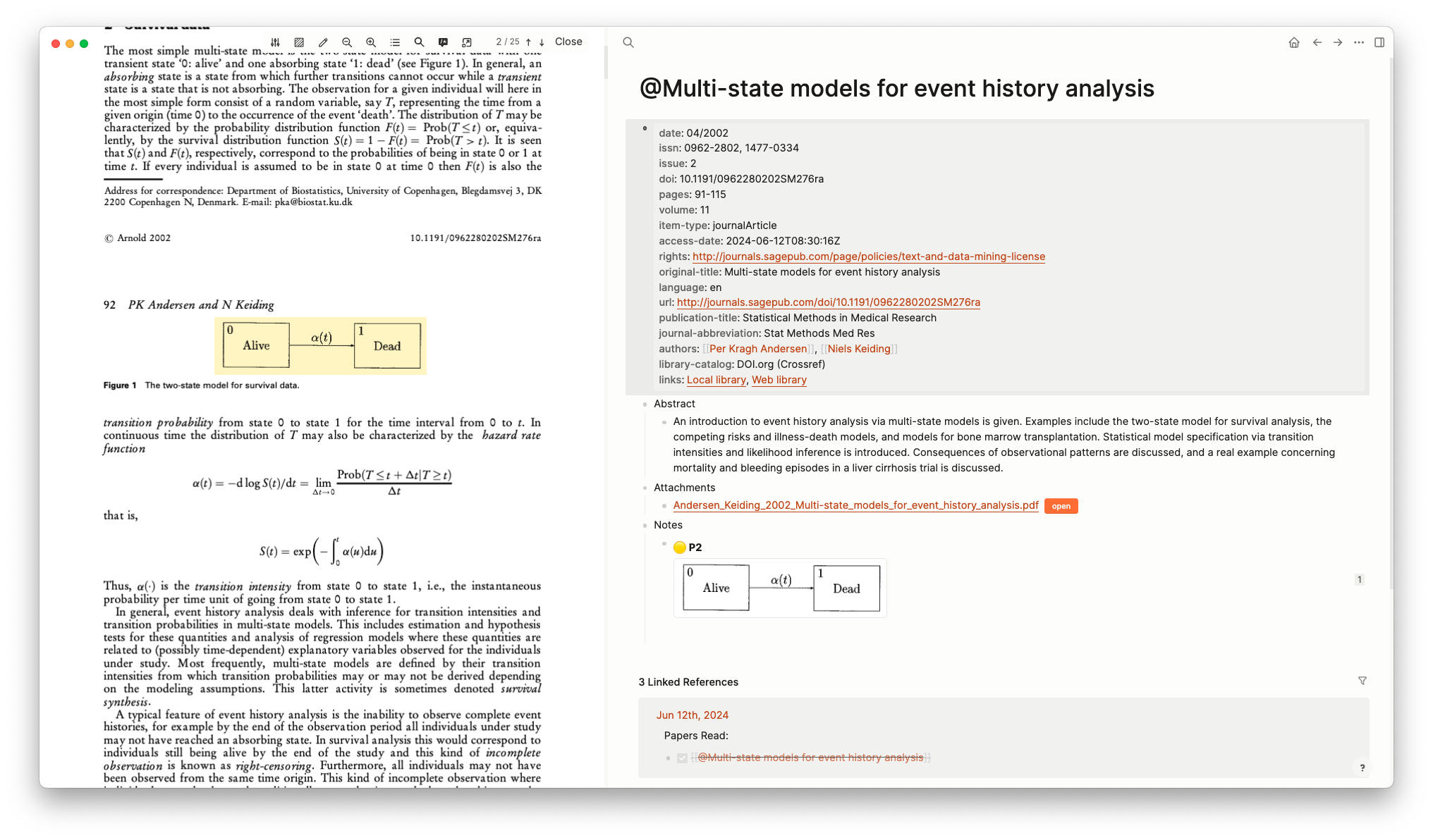
Logseq has built in support for the Zotero reference manager. This allowed me to import PDF files and easily extract their metadata, as well as make direct references to the PDFs I was reading. These references gave an image that that can be linked to on other pages using the block referencing described above. This was very useful when reading papers for the dissertation, and allowed me to quickly build up my knowledge graph with this information.

Isn’t it so sad⌗

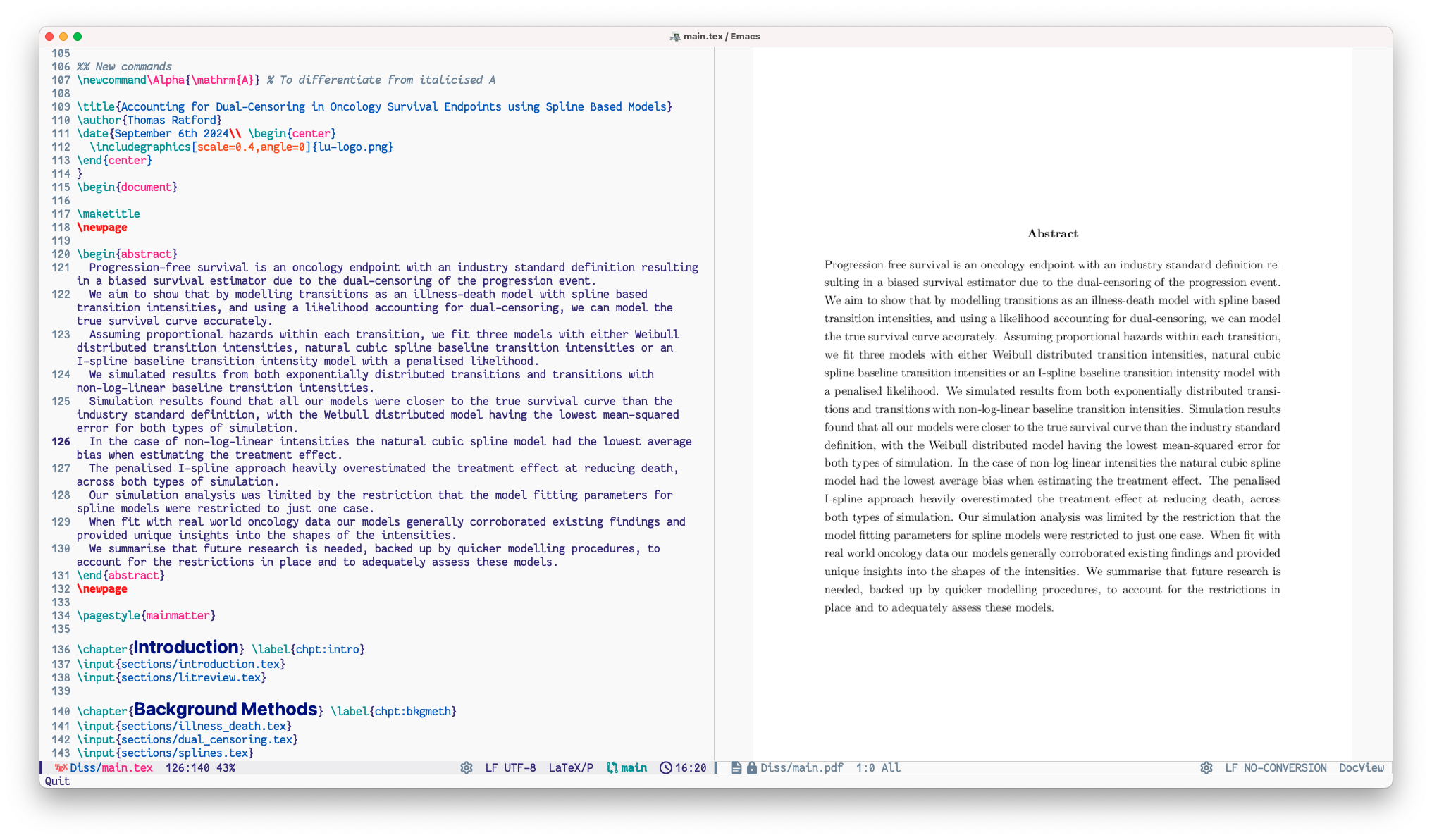
I wrote my dissertation, and all my coursework, entirely in \(\LaTeX\) using emacs. I used the auctex package for emacs to help with this, alongside the built-in doc-view package to view PDFs. My typical workflow was to open my .tex file and PDF simultaneously, and activate auto-revert-mode in the PDF buffer. This would then immediately reload the PDF upon any re-render of the \(\LaTeX\) file.

Auctex adds simple shortcuts to the latexmk and biber command line tools via C-c C-c (Ctrl+C twice). This gives a drop down of commands to compile the current open latex file or re-compute the bibliography; these compilation processes also provided useful hints on whether or not the PDF needed to be rerun again to ensure an accurate render. Overall I found the package to be very ergonomic and sped up my writing process immensely and I would highly recommend it to others writing in \(\LaTeX\). To make the dissertation (approx. 12,000 words) easier to read and edit, I separated out my disseration into smaller files for each section, before including into the main.tex file with \input{...}. In order for the auctex shortcut to render my main.tex file only, I had to add some small post-matter to each file

%%% Local Variables:
%%% mode: latex
%%% TeX-master: "../main"
%%% End:

In earlier coursework, I instead used a Makefile to build my latex files. This was primarily so that I could have autogenerating figures/values for each rerun, ensuring I was always using the most recent and correct values.

.PHONY: clean all figures

all: figures report.pdf

figures: main.R
	Rscript main.R

report.pdf: report.tex sources.bib
	latexmk -pdf --shell-escape -f report.tex

clean:
	rm -f report.bbl report.dvi report.fls report.aux report.aux.bbl report.aux.blg report.bcf report.blg report.log report.pdf report.run.xml
	rm -f figures/*

The main.R file included some small code to export plots and values, which could then be included with \input or \includegraphics.

log_output <-
  function(expr,
           filename = "figures/listing.Rout",
           append = F) {
    zz <- file(filename, open = ifelse(append, "a", "w"))
    on.exit(close(zz))
    sink(zz)
    try(expr)
    cat("\n")
    sink()
  }

plot_output <-
  function(p,
           filename = deparse(substitute(p)),
           width = 5,
           height = 5) {
    print(paste("sending to", filename))
    pdf(paste0("figures/", filename, ".pdf"),
        width = width,
        height = height)
    print(p)
    dev.off()
  }

# plot showing outlier
plot_output({
  with(MiniProj, {
    plot(x1, x3, xlab=expression(x[1]), ylab=expression(x[3]))
    points(x1[which(y == 1)], x3[which(y == 1)], col="#00FF00")
    points(x1[40], x3[40], col="red")
  })
}, filename = "obs40")

# average response value
log_output({
    cat(format(mean(MiniProj$y), digits = 3))
},"figures/mean.tex")

This allowed me to write The mean value of the response was \input{figures/mean} with confidence that the value would always be correct.

A brain that you’ve never had⌗